Basic (Gaussian likelihood) GP regression model

This notebook shows the different steps for creating and using a standard GP regression model, including: - reading and formatting data - choosing a kernel function - choosing a mean function (optional) - creating the model - viewing, getting, and setting model parameters - optimising the model parameters - making predictions

We focus here on the implementation of the models in GPflow; for more intuition on these models, see A Practical Guide to Gaussian Processes.

import gpflow
import numpy as np
import matplotlib

# The lines below are specific to the notebook format
%matplotlib inline
matplotlib.rcParams['figure.figsize'] = (12, 6)
plt = matplotlib.pyplot

X and Y denote the input and output values. NOTE: X and Y must be two-dimensional NumPy arrays, \(N \times 1\) or \(N \times D\), where \(D\) is the number of input dimensions/features, with the same number of rows as \(N\) (one for each data point):

data = np.genfromtxt('data/regression_1D.csv', delimiter=',')
X = data[:, 0].reshape(-1, 1)
Y = data[:, 1].reshape(-1, 1)

plt.plot(X, Y, 'kx', mew=2)

[<matplotlib.lines.Line2D at 0x7fe297f57cf8>]

We will consider the following probabilistic model:

\[ \begin{align}\begin{aligned}Y_i = f(X_i) + \varepsilon_i ,\\where :math:`f \sim \mathcal{GP}(\mu(.), k(., .'))`, and :math:`\varepsilon \sim \mathcal{N}(0, \tau^2 I)`.\end{aligned}\end{align} \]

Choose a kernel

Several kernels (covariance functions) are implemented in GPflow. You can easily combine them to create new ones (see Manipulating kernels). You can also implement new covariance functions, as shown in the Kernel design notebook. Here, we will use a simple one:

k = gpflow.kernels.Matern52(input_dim=1)

The input_dim parameter is the dimension of the input space. It typically corresponds to the number of columns in X (see Manipulating kernels for more information on kernels defined on subspaces). You can get a summary of the kernel, either by using print(k) (plain text) or as follows:

k.as_pandas_table()  #, or simply:
k

	class	prior	transform	trainable	shape	fixed_shape	value
Matern52/lengthscales	Parameter	None	+ve	True	()	True	1.0
Matern52/variance	Parameter	None	+ve	True	()	True	1.0

The Matern 5/2 kernel has two parameters: lengthscales, which encodes the “wiggliness” of the GP, and variance, which tunes the amplitude. They are both set to 1.0 as the default value. For more details on the meaning of the other columns, see Manipulating kernels.

Choose a mean function (optional)

It is common to choose \(\mu = 0\), which is the GPflow default.

However, if there is a clear pattern (such as a mean value of Y that is far away from 0, or a linear trend in the data), mean functions can be beneficial. Some simple ones are provided in the gpflow.mean_functions module.

Here’s how to define a linear mean function:

meanf = gpflow.mean_functions.Linear()

Construct a model

A GPflow model is created by instantiating one of the GPflow model classes, in this case GPR. We’ll make a kernel k and instantiate a GPR object using the generated data and the kernel. We’ll also set the variance of the likelihood to a sensible initial guess.

m = gpflow.models.GPR(X, Y, kern=k, mean_function=None)

You can get a summary of the model, either by using print(m) (plain text) or as follows:

m.as_pandas_table()  #, or simply:
m

	class	prior	transform	trainable	shape	fixed_shape	value
GPR/kern/lengthscales	Parameter	None	+ve	True	()	True	1.0
GPR/kern/variance	Parameter	None	+ve	True	()	True	1.0
GPR/likelihood/variance	Parameter	None	+ve	True	()	True	1.0

The first two lines correspond to the kernel parameters, and the third one gives the likelihood parameter (the noise variance \(\tau^2\) in our model).

You can access those values and manually set them to sensible initial guesses. For example:

m.likelihood.variance = 0.01
m.kern.lengthscales = 0.3

Optimise the model parameters

To obtain meaningful predictions, you need to tune the model parameters (that is, the parameters of the kernel, the likelihood, and the mean function if applicable) to the data at hand.

There are several optimisers available in GPflow. Here we use the ScipyOptimizer, which by default implements the L-BFGS-B algorithm. You can select other algorithms by using the method= keyword argument of ScipyOptimizer; see the SciPy documentation for details of available options.

opt = gpflow.train.ScipyOptimizer()
opt.minimize(m)
m.as_pandas_table()

INFO:tensorflow:Optimization terminated with:
  Message: b'CONVERGENCE: REL_REDUCTION_OF_F_<=_FACTR*EPSMCH'
  Objective function value: 9.733150
  Number of iterations: 20
  Number of functions evaluations: 22

INFO:tensorflow:Optimization terminated with:
  Message: b'CONVERGENCE: REL_REDUCTION_OF_F_<=_FACTR*EPSMCH'
  Objective function value: 9.733150
  Number of iterations: 20
  Number of functions evaluations: 22

	class	prior	transform	trainable	shape	fixed_shape	value
GPR/kern/lengthscales	Parameter	None	+ve	True	()	True	0.21241587062097605
GPR/kern/variance	Parameter	None	+ve	True	()	True	7.965730330409469
GPR/likelihood/variance	Parameter	None	+ve	True	()	True	0.005759487103521433

Notice how the value column has changed.

The local optimum found by Maximum Likelihood might not be the one you want (for example, it might be overfitting or oversmooth). This depends on the initial values of the hyperparameters, and is specific to each dataset. As an alternative to Maximum Likelihood, Markov Chain Monte Carlo (MCMC) is also available.

Make predictions

We can now use the model to make some predictions at the new points Xnew. You might be interested in predicting two different quantities: the latent function values f(Xnew) (the denoised signal), or the values of new observations y(Xnew) (signal + noise). Because we are dealing with Gaussian probabilistic models, the predictions typically produce a mean and variance as output. Alternatively, you can obtain samples of f(Xnew) or the log density of the new data points (Xnew, Ynew).

GPflow models have several prediction methods:

• m.predict_f returns the mean and variance of \(f\) at the points Xnew.

• m.predict_f_full_cov additionally returns the full covariance matrix of \(f\) at the points Xnew.

• m.predict_f_samples returns samples of the latent function.

• m.predict_y returns the mean and variance of a new data point (that is, it includes the noise variance).

• m.predict_density returns the log density of the observations Ynew at Xnew.

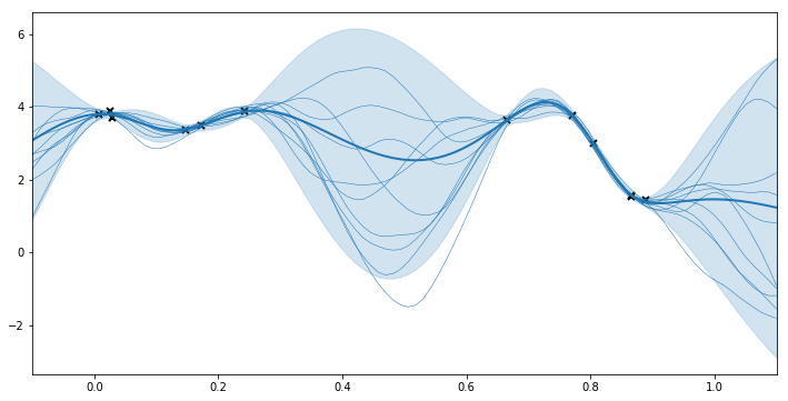
We use predict_f and predict_f_samples to plot 95% confidence intervals and samples from the posterior distribution.

## generate test points for prediction
xx = np.linspace(-0.1, 1.1, 100).reshape(100, 1)  # test points must be of shape (N, D)

## predict mean and variance of latent GP at test points
mean, var = m.predict_f(xx)

## generate 10 samples from posterior
samples = m.predict_f_samples(xx, 10)  # shape (10, 100, 1)

## plot
plt.figure(figsize=(12, 6))
plt.plot(X, Y, 'kx', mew=2)
plt.plot(xx, mean, 'C0', lw=2)
plt.fill_between(xx[:,0],
                 mean[:,0] - 1.96 * np.sqrt(var[:,0]),
                 mean[:,0] + 1.96 * np.sqrt(var[:,0]),
                 color='C0', alpha=0.2)

plt.plot(xx, samples[:, :, 0].T, 'C0', linewidth=.5)
plt.xlim(-0.1, 1.1);

GP regression in higher dimensions

Very little changes when the input space has more than one dimension. X is a NumPy array with one column for each dimension. The kernel can be set with input_dim equal to the number of columns of X. It is generally recommended that you set the ARD (Automatic Relevance Determination) parameter to True to enable you to tune a different lengthscale for each dimension.

Further reading

• Stochastic Variational Inference for scalability with SVGP for cases where there are a large number of observations.

• Ordinal regression if the data is ordinal.

• Multi-output models and coregionalisation if Y is multidimensional.