Manipulating GPflow models

One of the key ingredients in GPflow is the model class, which enables you to carefully control parameters. This notebook shows how some of these parameter control features work, and how to build your own model with GPflow. First we’ll look at:

• how to view models and parameters

• how to set parameter values

• how to constrain parameters (for example, variance > 0)

• how to fix model parameters

• how to apply priors to parameters

• how to optimise models

Then we’ll show how to build a simple logistic regression model, demonstrating the ease of the parameter framework.

GPy users should feel right at home, but there are some small differences.

First, let’s deal with the usual notebook boilerplate and make a simple GP regression model. See Basic (Gaussian likelihood) GP regression model for specifics of the model; we just want some parameters to play with.

import gpflow
import numpy as np

Create a very simple GP regression model wrapped in defer_build(). You must use defer_build() so that the model is not compiled in the TensorFlow graph, because adding transforms and priors is possible only for non-compiled models.

np.random.seed(1)
X = np.random.rand(20, 1)
Y = np.sin(12 * X) + 0.66 * np.cos(25 * X) + np.random.randn(20,1) * 0.01

with gpflow.defer_build():
    m = gpflow.models.GPR(X, Y, kern=gpflow.kernels.Matern32(1) + gpflow.kernels.Linear(1))

Viewing, getting, and setting parameters

You can display the state of the model in a terminal by using print(m), and by simply returning it in a notebook:

m

	class	prior	transform	trainable	shape	fixed_shape	value
GPR/kern/kernels/0/lengthscales	Parameter	None	+ve	True	()	True	1.0
GPR/kern/kernels/0/variance	Parameter	None	+ve	True	()	True	1.0
GPR/kern/kernels/1/variance	Parameter	None	+ve	True	()	True	1.0
GPR/likelihood/variance	Parameter	None	+ve	True	()	True	1.0

This model has four parameters. The kernel is made of the sum of two parts. The first (counting from zero) is a Matern32 kernel that has a variance parameter and a lengthscale parameter; the second is a linear kernel that has only a variance parameter. There is also a parameter that controls the variance of the noise, as part of the likelihood.

All the model variables have been initialised at 1.0. You can access individual parameters in the same way that you display the state of the model in a terminal; for example, to see all the parameters that are part of the likelihood, run:

m.likelihood

	class	prior	transform	trainable	shape	fixed_shape	value
GPR/likelihood/variance	Parameter	None	+ve	True	()	True	1.0

This gets more useful with more complex models!

To set the value of a parameter, just use an assignment statement:

m.kern.kernels[0].lengthscales = 0.5
m.likelihood.variance = 0.01
m

	class	prior	transform	trainable	shape	fixed_shape	value
GPR/kern/kernels/0/lengthscales	Parameter	None	+ve	True	()	True	0.5
GPR/kern/kernels/0/variance	Parameter	None	+ve	True	()	True	1.0
GPR/kern/kernels/1/variance	Parameter	None	+ve	True	()	True	1.0
GPR/likelihood/variance	Parameter	None	+ve	True	()	True	0.01

Constraints and trainable variables

GPflow helpfully creates an unconstrained representation of all the variables. In the previous example, all the variables are constrained positively (see the right-hand column in the table), the unconstrained representation is given by \(\alpha = \log(\exp(\theta)-1)\). read_trainables() returns the constrained values:

m.read_trainables()

{'GPR/kern/kernels/0/lengthscales': array(0.5),
 'GPR/kern/kernels/0/variance': array(1.),
 'GPR/kern/kernels/1/variance': array(1.),
 'GPR/likelihood/variance': array(0.01)}

Each parameter has an unconstrained_tensor attribute that enables you to access the unconstrained value as a TensorFlow Tensor (though only after the model has been compiled). You can also check the unconstrained value as follows:

p = m.kern.kernels[0].lengthscales
p.transform.backward(p.value)

-0.4327546710632299

Constraints are handled by the Transform classes. You might prefer to use the constraint \(\alpha = \log(\theta)\); this is easily done by changing the transform attribute on a parameter, with one simple condition - the model has not been compiled yet:

m.kern.kernels[0].lengthscales.transform = gpflow.transforms.Exp()

Though the lengthscale itself remains the same, the unconstrained lengthscale has changed:

p.transform.backward(p.value)

-0.6931491805619453

Another helpful feature is the ability to fix parameters. To do this, simply set the trainable attribute to False; this is shown in the trainable column of the representation, and the corresponding variable is removed from the free state.

m.kern.kernels[1].variance.trainable = False
m

	class	prior	transform	trainable	shape	fixed_shape	value
GPR/kern/kernels/0/lengthscales	Parameter	None	Exp	True	()	True	0.5
GPR/kern/kernels/0/variance	Parameter	None	+ve	True	()	True	1.0
GPR/kern/kernels/1/variance	Parameter	None	+ve	False	()	True	1.0
GPR/likelihood/variance	Parameter	None	+ve	True	()	True	0.01

m.read_trainables()

{'GPR/kern/kernels/0/lengthscales': array(0.5),
 'GPR/kern/kernels/0/variance': array(1.),
 'GPR/likelihood/variance': array(0.01)}

To unfix a parameter, just set the trainable attribute to True again.

m.kern.kernels[1].variance.trainable = True
m

	class	prior	transform	trainable	shape	fixed_shape	value
GPR/kern/kernels/0/lengthscales	Parameter	None	Exp	True	()	True	0.5
GPR/kern/kernels/0/variance	Parameter	None	+ve	True	()	True	1.0
GPR/kern/kernels/1/variance	Parameter	None	+ve	True	()	True	1.0
GPR/likelihood/variance	Parameter	None	+ve	True	()	True	0.01

Priors

You can set priors in the same way as transforms and trainability, by using members of the gpflow.priors module. Let’s set a Gamma prior on the RBF-variance.

m.kern.kernels[0].variance.prior = gpflow.priors.Gamma(2, 3)
m

	class	prior	transform	trainable	shape	fixed_shape	value
GPR/kern/kernels/0/lengthscales	Parameter	None	Exp	True	()	True	0.5
GPR/kern/kernels/0/variance	Parameter	Ga(2.0,3.0)	+ve	True	()	True	1.0
GPR/kern/kernels/1/variance	Parameter	None	+ve	True	()	True	1.0
GPR/likelihood/variance	Parameter	None	+ve	True	()	True	0.01

Optimisation

To optimise your model, first create an instance of an optimiser (in this case, gpflow.train.ScipyOptimizer), which has optional arguments that are passed to scipy.optimize.minimize (we minimise the negative log likelihood). Then, call the minimize method of that optimiser, with your model as the optimisation target. Variables that have priors are maximum a priori (MAP) estimated, that is, we add the log prior to the log likelihood, and otherwise use Maximum Likelihood.

m.compile()
opt = gpflow.train.ScipyOptimizer()
opt.minimize(m)

WARNING:tensorflow:From /home/st/anaconda3/envs/relaxedgp/lib/python3.7/site-packages/tensorflow/python/framework/op_def_library.py:263: colocate_with (from tensorflow.python.framework.ops) is deprecated and will be removed in a future version.
Instructions for updating:
Colocations handled automatically by placer.

WARNING:tensorflow:From /home/st/anaconda3/envs/relaxedgp/lib/python3.7/site-packages/tensorflow/python/framework/op_def_library.py:263: colocate_with (from tensorflow.python.framework.ops) is deprecated and will be removed in a future version.
Instructions for updating:
Colocations handled automatically by placer.

WARNING:tensorflow:From /home/st/anaconda3/envs/relaxedgp/lib/python3.7/site-packages/tensorflow/python/ops/math_ops.py:3066: to_int32 (from tensorflow.python.ops.math_ops) is deprecated and will be removed in a future version.
Instructions for updating:
Use tf.cast instead.

WARNING:tensorflow:From /home/st/anaconda3/envs/relaxedgp/lib/python3.7/site-packages/tensorflow/python/ops/math_ops.py:3066: to_int32 (from tensorflow.python.ops.math_ops) is deprecated and will be removed in a future version.
Instructions for updating:
Use tf.cast instead.

INFO:tensorflow:Optimization terminated with:
  Message: b'CONVERGENCE: REL_REDUCTION_OF_F_<=_FACTR*EPSMCH'
  Objective function value: 1.884455
  Number of iterations: 41
  Number of functions evaluations: 46

INFO:tensorflow:Optimization terminated with:
  Message: b'CONVERGENCE: REL_REDUCTION_OF_F_<=_FACTR*EPSMCH'
  Objective function value: 1.884455
  Number of iterations: 41
  Number of functions evaluations: 46

Building new models

To build new models, you’ll need to inherit from gpflow.models.Model. Parameters are instantiated with gpflow.Param. You might also be interested in gpflow.params.Parameterized, which acts as a ‘container’ for Params (for example, kernels are parameterised).

In this very simple demo, we’ll implement linear multiclass classification.

There are two parameters: a weight matrix and a bias (offset). The key thing to implement is the private _build_likelihood method, which returns a TensorFlow scalar that represents the (log) likelihood. You can use param objects inside _build_likelihood, but you need to use the constrained tensor attribute to access the tensor to use when building the graph (for example, self.kernel.variance.constrained_tensor).

Alternatively, decorate the function with @gpflow.params_as_tensors so that the objects appear as constrained tensors (for example, you can now refer to the TensorFlow object as self.kernel.variance rather than self.kernel.variance.constrained_tensor). This is useful when you are writing the model likelihood and dealing with the constrained_tensor attributes of several different Params, but note that you cannot access any of the other features of a Param object.

import tensorflow as tf

class LinearMulticlass(gpflow.models.Model):
    def __init__(self, X, Y, name=None):
        super().__init__(name=name) # always call the parent constructor

        self.X = X.copy() # X is a numpy array of inputs
        self.Y = Y.copy() # Y is a 1-of-k (one-hot) representation of the labels

        self.num_data, self.input_dim = X.shape
        _, self.num_classes = Y.shape

        #make some parameters
        self.W = gpflow.Param(np.random.randn(self.input_dim, self.num_classes))
        self.b = gpflow.Param(np.random.randn(self.num_classes))

        # ^^ You must make the parameters attributes of the class for
        # them to be picked up by the model. i.e. this won't work:
        #
        # W = gpflow.Param(...    <-- must be self.W

    @gpflow.params_as_tensors
    def _build_likelihood(self): # takes no arguments
        p = tf.nn.softmax(tf.matmul(self.X, self.W) + self.b) # Param variables are used as tensorflow arrays.
        return tf.reduce_sum(tf.log(p) * self.Y) # be sure to return a scalar

…and that’s it. Let’s build a really simple demo to show that it works.

np.random.seed(123)
X = np.vstack([np.random.randn(10,2) + [2,2],
               np.random.randn(10,2) + [-2,2],
               np.random.randn(10,2) + [2,-2]])
Y = np.repeat(np.eye(3), 10, 0)

from matplotlib import pyplot as plt
plt.style.use('ggplot')
%matplotlib inline
import matplotlib
matplotlib.rcParams['figure.figsize'] = (12,6)
plt.scatter(X[:,0], X[:,1], 100, np.argmax(Y, 1), lw=2, cmap=plt.cm.viridis);

m = LinearMulticlass(X, Y)
m

	class	prior	transform	trainable	shape	fixed_shape	value
LinearMulticlass/W	Parameter	None	(none)	True	(2, 3)	True	[[-0.7727087142471915, 0.7948626677932181, 0.3...
LinearMulticlass/b	Parameter	None	(none)	True	(3,)	True	[0.045490080631097156, -0.2330920609844135, -1...

opt = gpflow.train.ScipyOptimizer()
opt.minimize(m)
m

INFO:tensorflow:Optimization terminated with:
  Message: b'CONVERGENCE: NORM_OF_PROJECTED_GRADIENT_<=_PGTOL'
  Objective function value: 0.000013
  Number of iterations: 26
  Number of functions evaluations: 27

INFO:tensorflow:Optimization terminated with:
  Message: b'CONVERGENCE: NORM_OF_PROJECTED_GRADIENT_<=_PGTOL'
  Objective function value: 0.000013
  Number of iterations: 26
  Number of functions evaluations: 27

	class	prior	transform	trainable	shape	fixed_shape	value
LinearMulticlass/W	Parameter	None	(none)	True	(2, 3)	True	[[8.558497428410769, -30.636553276376564, 22.4...
LinearMulticlass/b	Parameter	None	(none)	True	(3,)	True	[11.857844278133033, -12.947434324958664, -0.2...

xx, yy = np.mgrid[-4:4:200j, -4:4:200j]
X_test = np.vstack([xx.flatten(), yy.flatten()]).T
f_test = np.dot(X_test, m.W.read_value()) + m.b.read_value()
p_test = np.exp(f_test)
p_test /= p_test.sum(1)[:,None]

plt.figure(figsize=(12, 6))
for i in range(3):
    plt.contour(xx, yy, p_test[:,i].reshape(200,200), [0.5], colors='k', linewidths=1)
plt.scatter(X[:,0], X[:,1], 100, np.argmax(Y, 1), lw=2, cmap=plt.cm.viridis);

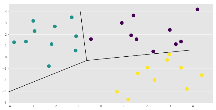
That concludes the new model example and this notebook. You might want to see for yourself that the LinearMulticlass model and its parameters have all the functionality demonstrated here. You could also add some priors and run Hamiltonian Monte Carlo using the HMC optimiser gpflow.train.HMC and its sample method. See Markov Chain Monte Carlo (MCMC) for more information on running the sampler.